Room EQ Wizard (REW) on OSX

Would you like to know if your speakers are placed poorly in your room? Are there room resonance interactions you can avoid? If so, Room EQ Wizard, known as REW, is a incredibly useful and free program written by John Mulcahy for room analysis. This post documents how to get it all up and running on a Mac. All of the following information is available on the internet, e.g. [1], [2], [3] and [4], but not in one place. 

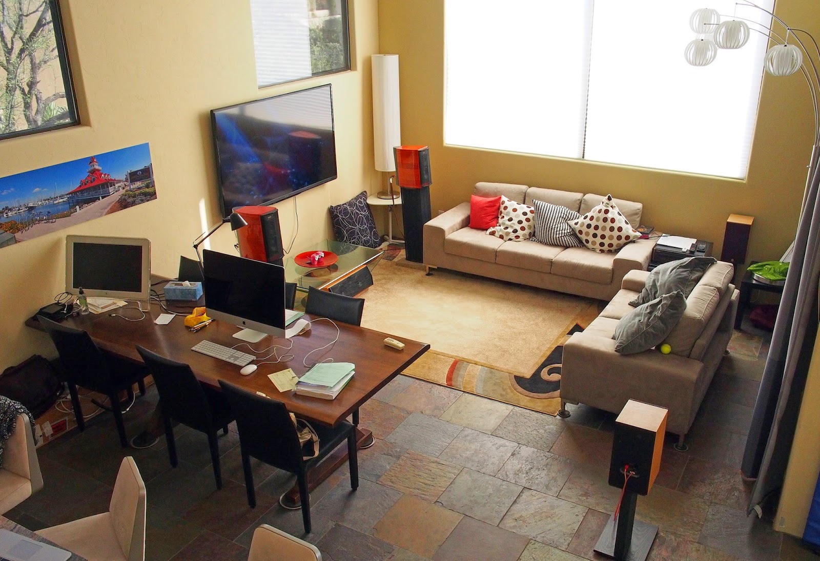
Sonus Faber Guarneri Mementos up front plus Cremona M center channel. Celestion SL-6 are my surrounds.

REW is written in Java. Version 5.0.1 beta 24 is the latest version at this time. (On Mavericks, Java Runtime Environment (JRE) 7 is installed by default but REW uses JRE 8.) However, REW runs fine under Mavericks (10.9) on my Macbook Pro. (I bet it runs fine under Yosemite (10.10) as well.) How? Well, it is bundled with and makes use of JRE 8 inside its own folder in Applications.

My laptop has a HDMI (digital) output that connects to my Pioneer receiver. The connection is necessary to route the test tones generated by REW to your speakers. A total of two cables are attached to my laptop, as shown below.

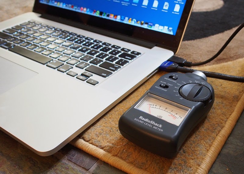
Macbook Pro. HDMI cable to receiver. USB cable to the UMIK-1 microphone. Radio Shack meter.

In addition, you will need:

1. A sound pressure meter for REW SPL calibration. (Set on C weighting and slow response.) Radio Shack has a cheap one for under $30. The classic one I got on sale (see pic above) is no longer available.



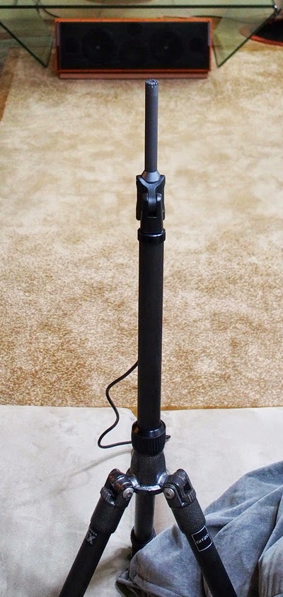
UMIK-1 mounted vertically via a Gitzo camera tripod at the listening position.

2. A calibrated USB microphone to pick up the test tones REW generates. The UMIK-1 is available from MiniDSP.com for $75. Conveniently, REW from version 5.0 onwards can auto-detect the UMIK-1. Cross-Spectrum sells a carefully calibrated version of this microphone for $100. I have the Cross-Spectrum UMIK-1 shown above. Notice that the microphone is positioned vertically in the picture above, and not pointing at any individual speaker. That's because we don't want to reposition the microphone for each individual speaker sweep. Although it's an omni-directional microphone, you need it calibrated specifically for this 90° position. Cross-Spectrum supplies the necessary calibration file.

Software-wise, you will also need a free program called Soundflower, a (virtual) audio middleman that allows you to route REW's output to the appropriate HDMI channel. First, plug in the HDMI cable to the receiver. In the Audio Midi setup app (found in Applications/Utilities), select HDMI. For output, format should be 48000.0 Hz.

In Configure Speakers... select the surround sound system you have. I have 5.1 surround selected. You can test if things are properly configured by clicking on each speaker icon and it'll play a test tone for a few seconds. All versions of HDMI have support for 8 channels of LPCM audio. By convention, HDMI channel 1 is the left front, channel 2 the right front, channel 3 the center speaker, channel 4 the subwoofer, and so on.

After Soundflower has been installed, start the Soundflower bed application. Once started, a cute flower icon at the top enables a pulldown menu. If the HDMI cable is connected (and selected by the receiver?), you can select HDMI for Soundflower (64ch) as shown below:

Then pairing Channel 1 with HDMI[1] will send REW test tones to the left front speaker. (To switch REW output to another speaker, just select the appropriate HDMI[X] channel.)

Selecting Channel 2 as None will silence REW for any other speaker.

Next, start the REW application. Assuming it's REW 5.0 or later, if the UMIK-1 microphone is plugged in, it should be able to see it and pop up the following messages:

Since the microphone is installed pointing directly upwards at the ceiling (see earlier picture), and we're not going to bother to (re-)point it at each speaker individually during measurement, use the narrow band response 90 degree calibration file supplied by Cross-Spectrum:

Once REW has started up, click on Preferences and check to see the output sample rate is 48 kHz and the virtual output device is Soundflower (64ch).

Explanation: REW will send the test tones to Soundflower and Soundflower will route it to the HDMI channel you've specified via the Soundflower bed pulldown menu above. Note that REW has already selected the input device to be the UMIK-1. I believe we're setting everything to sample at 48 kHz because the UMIK-1 is a 48 kHz native device (not all microphones are). The Input Volume (at 1.000 above) may need to be adjusted down if you need additional headroom; more on this later.

Next, click the SPL Meter button on the top row. Then click Calibrate on the REW SPL Meter.

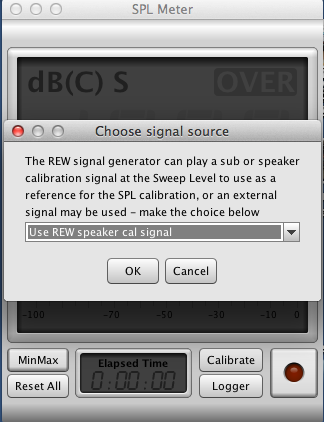
(I chose to use the speaker cal signal because I'm not currently running a subwoofer.)

REW will now send pink noise to your left front speaker.  Take the sound level meter and place it next to your microphone at the seating position.

Put it on C weighting (a mostly flat frequency response curve) and slow response (smoothed, 1 sec time constant). Set the sound level meter range dial to 80dB. Adjust your receiver volume until the physical meter reads 0dB, i.e. 80dB. Enter Finish. Then you should see something like the following message.

(To measure higher, the Input Volume field for the microphone, currently at 1.000, can be adjusted lower in REW preferences.)

The noise floor of USB-based microphones is about -50db. (Reality check: if the REW SPL meter is showing a much lower range, you have it adjusted wrong.)

Finally, it's time to do some measuring! Select Measure on the top row. Select for a sweep from 15 hz to 20,000 hz, and select Start Measuring:

(I'm not sure why people choose to begin early at 15Hz. First, the UMIK-1 specs are 20Hz-20kHz +/- 1dB. And, 15Hz (of course) is subsonic and not audible, although if you have a suitably impressive large speaker or subwoofer, it's feel-able.)

Anyway, you should get a graph like this when you click All SPL:

Note that the graph has been set to 15 hz to 20.0 kHz on the x-axis and 50 db to 90 db on the y-axis.

Actually, the initial plot will look a lot more jagged. 1/6 octave smoothing (selectable via the Controls button) is typically applied.

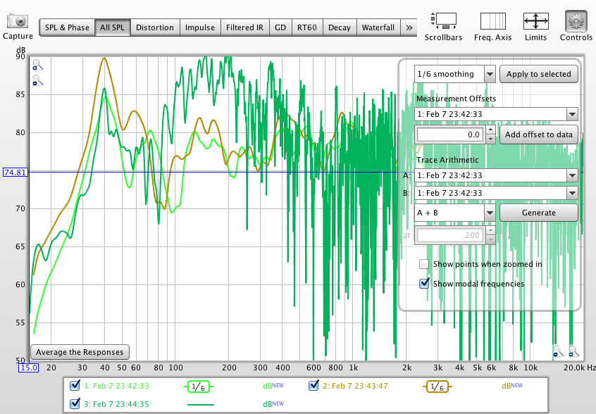
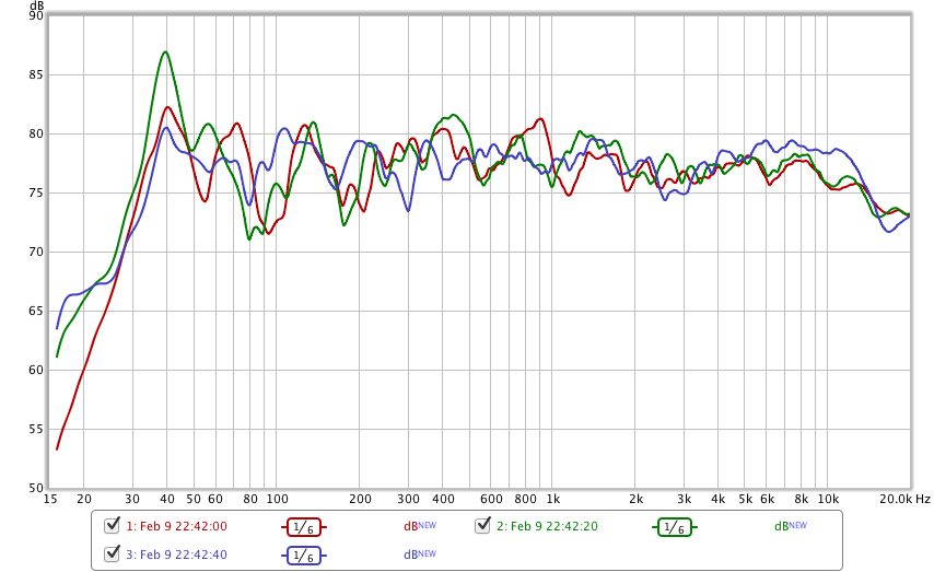
Three sweeps are overlaid. One from the front left speaker. one from the front right. And the unsmoothed sweep is from the center channel.

Once the preferred smoothing has been selected, click "Apply to selected". Here are the response curves from all front 3 speakers overlaid. 

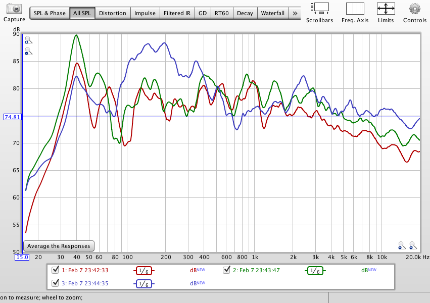
Red is front left speaker. Green is front right speaker. Blue is center speaker. Colors have been defaulted.

(Each time you conduct a sweep, by default it'll be plotted on top of the previous sweeps. Of course, you can choose to clear prior measurements.)

As you can see from the graph, there are some problems to be tackled. Even if you have room correction in the receiver, it'll be good to place the speakers and listening position as close to optimum as possible prior to (applying) room correction. 

Broadly speaking, my problems are: (1) there's a hump for all three speakers at 40 Hz. (2) the suckout around 80 Hz. (3) the 100-200 Hz broad bump for the center speaker. (4) the roll-off from 3 kHz on upwards for all three speakers. Could you have guessed all of these from the picture of my listening area (first picture above)? Not me. It's good to have the ability to measure the room/speaker combination!

Unfortunately, REW is not an AI program. It can't figure out the reasons for those non-linearities. To solve these one must experiment with positioning of the speakers (distances from the walls) and of the listening position (distance from the back wall). Also, one must calculate the room modes (which depend on the width, height and length of the room, assuming a simple rectangular shape).

With respect to the four problems, I've discovered so far:

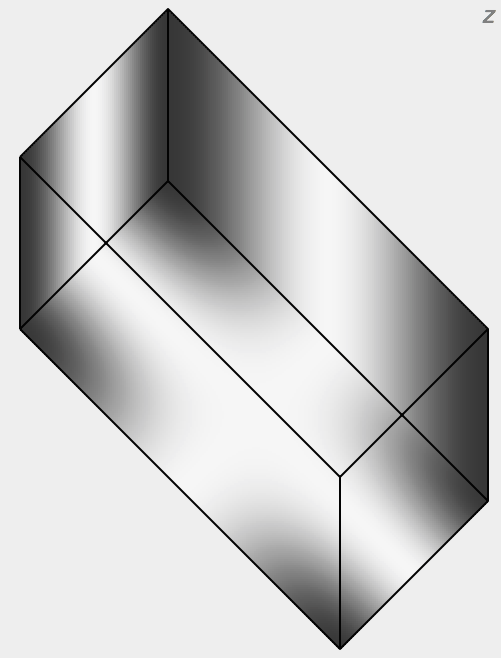
1. [40 Hz bump.] Something is responsible for the bump but it's not apparent (to me) from a simple, i.e. axial, analysis of the room dimensions. There is a good Room Eigenmodes calculator and sound pressure visualizer at [5]. Here is an example:

   

   Fundamental frequency standing wave representation. Dark = high sound pressure.

   Ceiling height at 12.5ft means f1 = 45 Hz because room height would be half a sine standing wave. (45 Hz is 1130 ft/sec (speed of sound) divided by 2 * 12.5 ft.) Length at 15ft means f1 = 38 Hz. It's not even clear what the room width is in my case because the left side is an open area. If I take the maximum width at 34 ft, f1 = 17 Hz, f3 = 50 Hz. There is a partial wall at 20.5 ft: if I use that, f1 = 28 Hz and f3 = 83 Hz. Doesn't coincide with 40 Hz. 

   

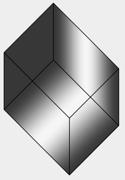
   41 Hz tangential mode for width 34ft and length 15ft 

   Looking at tangential modes, i.e. bouncing the sound waves off 4 walls instead of 2 parallel walls, there is a 41 Hz tangential fundamental mode that engages the full width, i.e. 34ft, and length of the room model. Perhaps that's what responsible for the 40 Hz hump. However, I believe that tangential modes are half as loud as (equivalent) axial modes. Most receivers have automatic room equalization built in. You can test if your receiver's auto-eq will attenuate that 40 Hz mode: surprisingly, mine doesn't seem to do anything, see below.
2. [Suckout at 80 Hz.] A major suckout is much more worrying. Room equalization can't do anything about it because it's presumably at a sound pressure null, and increasing amplifier power at that frequency band will only have minimal to no effect. Assuming the speakers are wired correctly with respect to phase, the only thing to do is experiment with varying the speaker and listening positions. Moving the speakers didn't seem to do anything. Fortunately, I discovered that moving the seating 1 foot forwards reduced the suckout substantially.
3. [100-200 Hz center speaker bump.] This one is easily corrected by the receiver. Perhaps it can also be mitigated by placing the center speaker higher or removing the glass table.
4. [3 kHz roll-off.] The speakers are pointing directly ahead. Tweeters can be quite directional. Toe in mitigated the roll off.

Applying toe-in and seating changes in conjunction with my budget Pioneer's unsophisticated MCACC system resulted in the following response curves:

Green: left front speaker. Red: right front speaker. Blue: center speaker.

More work is needed but you can see the frequency response of all three speakers have been improved. 40 Hz is also the port frequency for the Sonus Faber Guarneri, so there could be some interaction with the rear wall as the port exits out back. The right speaker has higher output than the left since there is a wall to its right, and the listening area opens out to a large area on the left. Low frequency response is non-existent due to the 6-inch woofers. A subwoofer would change things dramatically below 40 Hz.

References

1. Using the UMIK-1with REW and HDMI output - Mac. http://www.minidsp.com/applications/acoustic-measurements/umik-1-hdmi-on-mac

2. Room EQ Wizard on the Mac - An input workaround. http://johnr.hifizine.com/2013/02/room-eq-wizard-on-the-mac-an-input-workaround/

3. Workaround for 8 channel HDMI out on the Mac. http://www.hometheatershack.com/forums/rew-forum/69754-workaround-8-channel-hdmi-out-mac.html

4. Getting Started with REW. http://www.roomeqwizard.com/REWV5_help.pdf

5. Room Eigenmodes Calculator. http://www.hunecke.de/en/calculators/room-eigenmodes.html

Life journey: Days of Future Passed

Days of Future Passed.

A famous writer once said: "a journey is like marriage. The certain way to be wrong is to think you control it."

Or marriage is like a journey... 

My sincere hope is that we walk the downhills and uphills... 

together, or at least take the tandem... :)

The da Vinci JointVenture tandem

Background

In late 2013, I was ready to order a decent quality tandem, something mid-range. We'd already had experience renting tandems in places like Martha's Vineyard and Hangzhou as a great way of sightseeing around the island and the famous West Lake, respectively.

Hangzhou's West Lake

Tandem rental place in Hangzhou. Note the shade on some of the tandems. Very welcome when it's 108F and sunny.

West Tisbury, Martha's Vineyard

Gay Head cliffs, Aquinnah, Martha's Vineyard

A Visit to Denver

On Thanksgiving weekend, we decided to combine a Denver ski trip (to Winter Park) with a visit to da Vinci Designs. Their claim to fame is building tandems with an ICS (Independent Coasting System).

(Some years back, I did a couple of brevets on a conventional tandem (Santana), and I've always hated the idea that I couldn't stop pedaling when I wanted.)

However, I didn't want to spend the money without taking a test ride. So after one day of skiing, we went downtown Denver and test rode a lower end ICS tandem along the South Platte River Greenway.

Greenway near the Sports Authority Mile High stadium

We test rode a Grand Junction, courtesy of Todd Shusterman. Note the cold weather gear; it's late November in Denver.

The Grand Junction is a lower-end model built in Taiwan. It still has the ICS.

We also got a factory tour. Some pictures:

Frames are specific to da Vinci Designs since they need that extra bottom bracket on top of the bottom tube for the ICS plus the small tube that holds the front derailleur.

Close up of the head tube.

A stable of tandems, some carbon-fiber, mostly steel, available for test rides.

The ICS requires three chains. The incalculable benefit is the stoker is able to coast independently from the captain.  Plus four chainrings on the front. The downside is additional complexity and weight.

Frame tubes in steel, aluminum and carbon fiber.

Selecting a Tandem

We decided on a JointVenture, da Vinci's second-from-the-top model. And on aluminum as a compromise for the frame material: aluminum is considerably less expensive than titanium or carbon-fiber and a bit lighter than steel. It's a $400 up-charge though. Finally, we decided on the 26" wheel size, as opposed to 700c.  Being only 5'8" tall, I find the 650c wheel size works nicely for me on my regular road bike, a custom Litespeed Ghisallo. Given these frame parameters (aluminum, 26" wheel, small frame), it turns out a suitable frame was already available and hanging on the wall:

Unpainted frame. Ours is the first one.

Todd holding our frame. Notice that weld!

Next, we decided on the color combination, an extra-cost, top-to-bottom two-color fade:

Difficult palette decisions: violet on top or blue on the bottom?

Looking to see how the colors look in sunlight.

Like buying a new car, the base price can quickly get out of control if you start adding packages and special options. To keep the cost from spiraling too far, we decided on just upgrade package #2, which included the Wound Up carbon fork, front disc brake, the two-color fade, and upgraded bits for the ICS and headset. The drivetrain is uniquely interesting. We opted for Campagnolo (over Shimano) shifters as enables the front derailleur to have four chainrings in front (equiv. to 24T, 36T, 48T, and 60T). On the back there is a 11-32 9-speed cluster.

Delivery

There are a bunch of other details to be nailed down but I was ready to confirm the order about a week after Thanksgiving and put down a 50% deposit. Only thing I didn't really want was their choice of captain's saddle, since I had a couple of (my preferred) Selle Italia SLR saddles stashed away. 

In mid-January, we got a call from da Vinci Designs saying that they were about ready to ship. The phone conversation ended up with swapping out a couple more of their stock components for a 42cm 3T Prima 199 handlebar paired with a Ritchey WCS 110mm stem. Plus a Bontrager carbon seat post. Fortunately, that added only another $25 to the total. 

Shipping was another $150 from Denver. Anyway, last Friday the Fedex truck came by with a 2.1 meter long box:

Even without the front wheel attached, it came in a very long cardboard box.

Some self-assembly is required. It also comes without pedals; we decided to use low-end (double-sided) Shimano SPD mountain bike pedals for robustness and walkability. I spent the morning slowly documenting the unwrap (should I need to repack the bike), and installing the front and rear handlebars, the front chain, the front disc brake and wheel.

Assembled and ready to go for a ride.

I forgot to buy waterbottle cages. It has mounts for 5 (five!) cages on the frame. Including the 4 cages, the bike comes to 35 lbs.

Maiden Ride

The first shakedown ride was on a 20 mile rolling loop popular with locals. The disc brakes were disconcertingly weak and squealed like a proverbial pig being dragged off to slaughter first time around, but settled in quietly afterwards. With 200mm rotors, there is plenty of stopping power.

Rancho Vistoso Blvd.

We are looking forward to many more rides on our JointVenture...

Appendix

Spec sheet as far as I can figure out.

Nike+ and Matlab: part 2

In an earlier post, I described my first efforts at writing functions for using my iPod Nano with Matlab (here). As I pointed out, that wasn't functionality that I was really missing; in other words, I could do the same with Excel, though not with the Nike+ website.

Because that Matlab is such a powerful interactive and programming tool, it's easy to add functionality when you think of a new need. For example, yesterday I ran for 36 minutes, divided into a 10 min easy warm-up, and 26 mins at pace. The Nike+ website gives me:



which doesn't quite reflect the nature of my workout. Instead, what I want is the following:



This graph makes a lot more sense. You can see I have marked the average speed for both the first 10 mins (10.4 km/h) and the subsequent section (11.9 km/h) separately. I have overlaid the plot (raw and smooth) with the averages for the two sections as horizontal lines in blue.

To plot the recorded data, I simply call the nike function from last time:



Note, I've modified the call (and code) a bit to return both the number of data points collected and the array itself. (This is because I'm going to massage the data a bit.) At this point, I notice that there are a few blips in the data. There are two recorded data points that say I'm running at 60 and 80 km/h, respectively - which of course, is absurd. These data points will affect the average speed recorded, so I'll want to remove them by running another function that I wrote for the purpose, called rmoutliers:



It returns n, the number of outliers detected, and the modified array (a). Here, n=2 and all is well. How did I define what constitutes an outlier? Well, I crudely decided that 3 standard deviations away from the mean would count. Here is the code:



Notice I simply decided to replace those outlier points with the mean. (I could do something different and a bit more realistic, like use a moving average, of course.)

Finally, I want to overlay my average speed for the first 10 minutes and the rest of the run. We can add another function plotavg as follows:



I wrote this to say plot the average for mins 0 through 10. And then the average for mins 10 through 36. And in both cases, tell me what the average was for the defined segment. The code is very simple:



The end result is:



This functionality is simply not possible using a program with a simple, fixed menu of options because there will always be more things you'd like the program to have that you didn't think of initially. And one might be reluctant to dig into code and recompile an updated application just for one more function. But because Matlab is so programmable, these tasks are easy to do even on one-time basis.

Learning by doing: Nike+ and Matlab

I subscribe to the view that the best way to learn a complex and powerful tool or programming language is by doing.

Matlab is particularly nice for dealing with quantitative data. I decided to dive deeper into the tool by coding up a graphing application for my treadmill workouts recorded using the Nike+ application that samples data from the built-in accelerometer of the iPod Nano.

This is not necessarily functionality that I'm currently missing; normally I use Excel or the Nike+ website (based on Adobe Flash). Perhaps Matlab is overkill, but there's something deeply satisfying about smoothing the accelerometer data using just one function call like:

c = smooth(b);

where b and c are vectors. The default is a simple moving average (span 5). But because it's Matlab, you can play with many different smoothing options:

I'm looking to produce a graph like this automatically:

We have three graphs overlaid on top of one another; I'm plotting speed against time:

1. the raw data (in gray),
2. the smoothed data (in thick red), and
3. the treadmill speed setting (in blue)

When the iPod Nano is attached to my Mac, the raw xml file for my workout looks something like this:

The Nano records a datapoint, the cumulative distance in km, every 10 seconds.

We can grab those raw distances between the <extendedData dataType="distance"> and </extendedData> tags using a simple 3 line Perl program, as Matlab is perhaps not the best tool for this job:

The cool thing though is that Matlab can call Perl to stick the distances in a file (distances.txt):


perl('getdistances.perl',f)


Then we can call the importdata function to read those distances into an array (a):


a = importdata('distances.txt');


To extract the speeds in km/h units, we do a little conversion from our raw cumulative distances in km/10 sec units. It's a shame that the MuPad (symbolic math) part of Matlab is not well-integrated with Matlab proper because the unit::convert system there is cool. For example, you can define your own units like km/10 sec. (Anyway, I couldn't figure out how to make MuPad and Matlab work together.) Fortunately, the function convvel (convert velocity) can do km/s to km/h.

Finally, the rest is just plotting the data points. Setting a few labels and the ticks on the graph. I packaged this whole sequence up in a function called nike and saved it in Documents/Matlab/nike.m:

To use the graphing, I just call the function nike with the xml filename recorded by the iPod. (Matlab knows to look for this function in Documents/Matlab by default.) The call to nike (see below) returns the number of data points (181).

And up pops this graph:

This only works well when I have Matlab already open. For some reason, on my Macbook Pro, Matlab takes forever to start up.

There is a second call above to a function called treadmill, which handles the overlay of my treadmill program onto the iPod data.

I supply a vector [7,15,7.5,5,7,5,7.5,5] describing my workout: this means first 7 mph for 15 mins, followed by 7.5 mph for 5 mins, followed by 7 mph for 5 mins, and finally, 7.5 mph for 5 mins, for a total of 30 minutes. Note this is America, so the treadmill is in mph and I use convvel again to flip the values to km/h. Function implementing this is stored in Documents/Matlab/treadmill.m:

And I get my overlay:

Now, what's also cool about Matlab is that it's both interactive and programmatic. So, after running those two functions, I can simply click on the y-axis and zoom into where I want, resize the graph, add a few more labels, and put up a legend. The result:

So nice and easy.

Actually, the Adobe Flash-based graph from the Nike+ website is not bad either (although we can't have overlays):